Home » CBSE 9 » GRAPHICAL REPRESENTATION OF EQUATION OF MOTION

GRAPHICAL REPRESENTATION OF EQUATION OF MOTION

July 5, 2021
By Subham

So we come to the main topic of motion that is graphical representation of equation of motion. In this section we will learn, how we will established the equation of motion graphically. For that, in my previous post we learned about how we can plot ” Distance time graph ” and ” Velocity time graph “.

Let we see in this post how we can established equation of motion graphically. Here we can see how easily we can prove all laws of motion graphically.

v = u + at
s = ut + $\frac{1}{2}$ at²
v² = u² + 2as

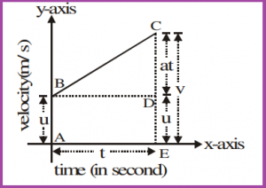
Here in above diagram, as we see it is a velocity-time graph BC, in which AB represents the initial velocity u, CE represents final velocity v, such that the change in velocity is represented by CD, which takes place in time t, represented by AE. From above diagram we can easily understand graphical representation of equation of motion.

Derivation of v = u + at

As we know the slope of a velocity time graph represents acceleration.

So we can say,

Acceleration = slope of the graph line BC.

$a=\frac{CD}{BD}=\frac{CE-DE}{BD}$ $\begin{vmatrix} DE=AB=u; &BD=AE=t; & CE=v \end{vmatrix}$

$a=\frac{v-u}{t}$

v – u = at

v = u + at

Derivation of s = ut + $\frac{1}{2}$ at²

The area enclosed by velocity time graph represents distance.

so,

Distance traveled = Area of trapezium ABCE =
Area of rectangle ABDE + Area of triangle BCD $\begin{bmatrix} BD = AE = t\\ CD = CE-DE = v - u\\ \end{bmatrix}$
= AB × AE + $\frac{1}{2}$ (BD × CD) = t × u + $\frac{1}{2}$ [t × (v–u)] $\begin{bmatrix} a = \frac{v - u}{t}\\ v - u = at \end{bmatrix}$

= ut + $\frac{1}{2}$ [t x at]

S = ut + $\frac{1}{2}$ at²

Derivation of v² = u² + 2as

As we know, the area enclosed by velocity time graph represents distance.

so,

From the velocity-time graph distance covered = Area of trapezium ABCE
⇒ S = $\frac{1}{2}$ (AB + CE) × AE

S = $\frac{1}{2}$ (u + v) × t …………………………….(i)

$Acceleration = \frac{Change in velocity}{Time}$

$a = \frac{v - u}{t}$

$t = \frac{v - u}{a}$

Substituting the value of t in eq (i)

S = $\frac{(v + u)}{2} + \frac{(v - u)}{a}$

S = $\frac{v^{2} - u^{2}}{2a}$

v² – u² = 2as

Finally here you can see complete video lecture on graphical representation of equation of motion for CBSE class 9 students.

Let’s check how you learn Graphical Representation of Equation of Motion ?

[WpProQuiz 6]

You may read those too…..

Not Enough, Need More

Subham

Hi myself Subham Dutta, having 15+ years experience in filed of teaching. I love to teach and try to build foundation of students. Try to make them imagine what they learn.